Buffon’s Needle
Buffon’s Needle is a problem first posed by the French naturalist and mathematician, the Comte de Buffon (1707-1788). Consider a plane, ruled with equidistant parallel lines, where the distance between the lines is D. A needle of length L is tossed onto the plane. What is the probability that the needle intersects one or more lines. The original problem had the condition that L < D, but in this version, we will also consider the probability where D ≤ L. With no more information than this, we have no way of knowing which part of the plane the needle is most likely to fall on. We do not know if the orientation of the needle is affected by the orientation of the lines, or by the needle’s location. Since we do not have this information, we can only assume that there are no such predictable relationships. Next, we must define appropriate random variables.
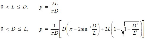
0 < Y ≤ D 0 < Θ ≤ π When plotted on the θ‑y plane, the pair (Θ, Y) is distributed over a rectangle with width π, and height D. We are assuming that the random variables, Θ and Y, are independent and uniformly distributed. Both of these conditions are important. If they are met, then the variables’ joint distribution is uniform. All subregions of equal area have equal probability of containing the point (Θ, Y). We now must define the region representing successes. The probability is the ratio of the area of the success region to the area of the region of distribution. The websketch below is interactive. The needle may be translated by dragging the blue endpoint. It may be rotated by dragging the green endpoint. As the ends of the needle are moved, you will observe changes in the red dot, which represents (Θ, Y) on the θ‑y plane. The slider below the graph controls the length of the needle. The blue rectangle on the graph represents the region of possible outcomes for (Θ, Y). The upper end of the needle is LsinΘ above the lower end. The needle will intersect the line if this value is greater than or equal to Y, that is, if the point (Θ, Y) falls on or below the curve y = Lsinθ. This curve is plotted on the graph, shown here with D < L. Any point in the shaded region below the curve and within the rectangle represents a success. This can be verified by manipulating the ends of the needle. If the needle crosses the line, the red point will be in the region of success. The probability of success may be computed by dividing the area of the success region by the area of the rectangle. Note that if D < L, then part of the curve leaves the rectangle. This is why we need a different, more complex formula for that situation. Not all of the region below the curve falls within the rectangle. We cannot consider the success or failure of coordinates which are not even possible to achieve. Either formula is applicable when D = L, the limiting case. The computed area is derived from these formulas:
How were the formulas derived? The exact area of the region of success may be computed by integration. This is left as an exercise. When D < L, that region must be divided into three parts, so be careful. The probability is that area divided by the area of the rectangle, πD. A Simulation Below is a simulation of the experiment with 1000 needles. The line spacing and needle length may be adjusted. The actual results are represented with the red and green vertical bars on the thermometer scale. A horizontal line across that scale represents the computed theoretical probability. Further Investigations: These results may be verified by conducting an experiment. I once did this in a class. The floor of the classroom was covered with 9" square tiles in a grid. We used tile joints to represent the parallel lines. For needles we used 9" dowells. The class paired off, and each pair of students conducted one hundred needle tosses and recorded the results. In this experiment, L = D, so we would expect the number of successes to be about 2/π times the number of trials. How could we use the results to compute an estimate for π? This experiment could have been simulated with a spreadsheet or some other computer program. Write a simulation and see how it fits. During the experiment, one pair of students saw a way to cut their work by half. The tiles formed a square grid, with two sets of parallel lines, one set running north-south, and the other set running east-west. Instead of tossing one hundred needles, they tossed only fifty, but they checked them against both sets of lines. They reasoned that the direction of the lines did not affect the probability. Therefore, each toss of a needle could represent two trials. Was their reasoning sound? Had they in fact simulated one hundred independent trials, although they only tossed fifty needles? Would they have the same expected number of successes? If you were able to compute the probabilities above, try this variation. Suppose we consider both sets of lines in the square grid. What is the probability of the needle crossing one or more lines? Consider two general cases, 0 < L ≤ D, and Follow-up The first case, where L ≤ D, should be within the grasp of a beginning calculus student. You only need to be able to compute the area of the rectangle, and integrate to get the area beneath the curve. The solution for D < L is a bit more involved. Three years after publishing this analysis, I did a write-up of the solution for the second case. Web Sketchpad FilesThe animated sketches on this page were created with Web Sketchpad, a developmental version of The Geometer’s Sketchpad. Copyright © 2024 KCP Technologies, a McGraw-Hill Education Company. All rights reserved.
Exported 4/7/2026 11:51:15 PM by GSP 5.11B3062(dev) (3062(dev))
Back to Whistler Alley Mathematics Last update: May 27, 2026 ... Paul Kunkel whistling@whistleralley.com For email to reach me, the word geometry must appear in the body of the message. |
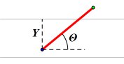 Orient the plane so that the parallel lines run horizontally. Now consider the lower end of the needle. If the needle is horizontal, it will not have a lower end. In that event (which has a probability of zero), choose the right end. Let Y be the distance from the lower end to the nearest line above it. We need not consider its horizontal position because a change in that direction would have no effect on the problem. And since the lines are equally spaced, it does not matter which lines the needle falls near. Now let the needle’s orientation angle, Θ, be defined as shown in the diagram. It may have a value ranging from zero (right) counterclockwise to π (left). Θ cannot be greater than π, because then the vertex of the angle would no longer be the lower end of the needle.