The Planimeter

The planimeter is a drafting instrument used to measure the area of a graphically represented planar region. The region being measured may have any irregular shape, making this instrument remarkably versatile. In this age of CAD and digital images, I suspect that the planimeter is heading toward obsolescence, but not just yet. They are still being manufactured.

When I first used a planimeter, I was somewhat troubled by the fact that I did not understand how it worked. Oh sure, I don't understand how my car works either, but the planimeter essentially has only three moving parts. That makes its mechanism considerably less complex than a typical doorknob. After eighteen years of sleepless nights, I decided to buy a planimeter and figure it out.

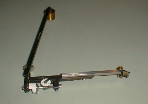
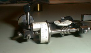
This is my planimeter. I got it at a Snohomish antique mall. It was made in Germany and distributed by Keuffel and Esser. The date on the bottom of the box says 1917. It is in perfect working condition, and it is nearly identical to the instruments I was using in the early 80s. The brass cylinder is anchored to the table with a point, like a compass point. It pivots, but does not slide. The elbow joint bents and slides freely. The pointer on the other end is used to trace the perimeter of the region. Near the elbow is a wheel, which simply rolls and slides along the tabletop. The scale is on the wheel itself, so it tells how far the wheel has turned. Sure enough, that number is proportional to the area of the region. The conversion factor depends on the scale of the drawing or photograph.

Here is a schematic of the instrument. If your browser supports Java, you can click on it and go to an interactive sketch, allowing you to get the feel of it. Point A is stationary. Point C traces the region in a clockwise direction.

The scale wheel is attached to the "green" arm, near point B, and its axis is parallel to the green arm, BC. This orientation is important. Suppose that the green arm has a translational motion. That is, it slides but it is always pointed in the same direction. If it moves longitudinally, then the wheel will not turn at all. It will merely slide sideways. If the arm moves in any other direction, then the rotation of the wheel will be proportional to the component of the translation that is normal to BC. Also, it would not matter where the wheel is attached, as long as it stays fixed to the green arm, with its axis parallel to BC.

You probably noticed that these conditional statements are not realistic. The green arm most certainly does not always point the in the same direction. It rotates as it moves. Just stay with me on this one. We are going to start with some simple cases.

I have confirmed, mathematically and experimentally, that the length of the blue arm, AB, is irrelevant. That length must be constant, but the results will be the same no matter what the length is. Again, humor me on this, at least for now. Point A is fixed, and AB is some fixed distance, so the blue arm acts as a compass, and point B travels along a circle. Since the distance AB does not matter, let point A be sent a very long distance away. As A approaches a point at infinity, the arc traced by point B approaches a line.

Let M be the final reading on the wheel, so M must be the sum of the measurements made on the four sides.

Multiply that measurement by k, the length of the green arm.

Now do you see where this is going? The yellow and blue parallelograms can be mapped to rectangles without changing their areas. Take the difference of their areas, and we are left with the area of rectangle PQRS.

What was proved here?

I know, I know. It looks like a lot of hand waving so far. The planimeter in this model does not even have the same construction as the one in the picture. I said that I would get back to that, and I will, but not right now. Also, I said that this instrument would measure the area of irregularly shaped regions, but I only proved that my modified instrument (which is called a linear planimeter) would work for a rectangle that is oriented square with the runner. What about that irregular region?

Refer to the region below, with the sinuous boundary. A nice thing about rectangles is that they can be stacked together in such as way that they will tile a plane, leaving no gaps between the rectangles. There are gaps between the rectangles and the blue boundary, but by constructing smaller and smaller rectangles, those gaps become as small as we wish.

Now, using the linear planimeter, trace one rectangle. Lift the planimeter so that the wheel does not move. Place it down on a second rectangle, and trace it. Continue doing this until all of the rectangles have been traced. The scale will show an accurate area for the region.

This process will work, but it is not at all practical. There is too much lifting and moving. Fortunately, there is a way to simplify the routine. Notice that each of the interior line segments was traced exactly twice. In fact, they were traced in opposite directions, effectively canceling any change in the instrument's scale. That means that we could just as well skip all of the interior courses.

What we need to be tracing is the perimeter courses, highlighted in red here. Of course, it would be more accurate if we fill in those gaps with smaller rectangles. As we fill more and more of the gaps, this red boundary takes the shape of the original boundary. In other words, we could save a lot of work by forgetting all of the rectangles and simply tracing the boundary. That is exactly how a planimeter is used.

But what about a polar planimeter?

This part is being saved for last because it requires calculus. If you are willing to accept my word that the length of the blue anchor arm does not matter, then the explanation above may give you a conceptual understanding of the planimeter.

In this sketch we have a planimeter tracing a boundary. Notice that the path of point B is restricted to a circle. For now, forget about the area of the region. Concentrate on the area that is covered by the green arm. Take the arbitrarily small subregion covered as the planimeter goes from C to C'. Call its area dw.

We know how to compute the area when the green arm is sliding, but in this case, it is sliding and turning at the same time. It will help to separate the components of this motion. First let the arm pivot, so that it is parallel to B'C'. Construct point E to show this first step. Now let the arm slide the rest of the way to B'C'. The subregion is now shown as a pentagon, BCEC'B'.

Let dθ be the rotation of the arm as it goes from C to E. Let dm be the change in the scale reading only while the arm is sliding. The scale also moves when the arm rotates, but that will be addressed later. As before, k is the length of the green arm. The area of the subregion can now be expressed algebraically. Some of these area formulas may appear to be approximations, but remember, both dθ and dm are arbitrarily small.

By integrating as the planimeter traces the entire region, we can get a formula for W, the area of the region crossed by the green arm when the planimeter makes one complete circuit around the region.

The first term in this formula integrates the angle change as the pointer traces the entire region. Since the planimeter begins and ends in the same position, the net change in the angle is zero. Therefore, the changes in the scale reading caused by rotation have no influence on the final reading.

Remember that dm was defined as the movement of the scale due to the sliding of the arm. This is the only thing reflected in the area equation. The integration of dm over the entire circuit is simply the net change in the scale, in other words, the final scale reading. Let M be the final scale reading.

Of course, what we computed was the area crossed by the green arm, not the area of the region that was traced. Think again. When the arm is sliding backwards, the scale is moving backwards. In that case, the area it is covering is subtracted from the total. When the planimeter traces a region, the arm makes a broad sweep, then backs over the part that is outside of the region.

In fact, some of the parts may be covered more than twice. Work it out. The exterior region will be covered an even number of times, alternating signs each time. The interior is covered an odd number of times, with a net equivalent of being crossed once in the positive direction.

There is still one more loose end. As I said earlier, the length of the blue arm is immaterial, and I proved it mathematically and experimentally. For the experimental part, I simply taped an extension onto the arm and compared the results. How was it proved mathematically? Go back through the calculations. At no time did we need to specify the length of the blue arm. If we can compute the area without knowing the arm length, then it does not matter what that length is. However, the length must be constant (Why?), and of course, the pointer must be able to reach all points on the boundary.

Will the planimeter work if the anchor point is within the region being measured?

Why or why not?

German Adaptation

Content from this page has been adapted and merged into a German language article by Wolf-G. Blümich. It can be accessed at the link below.

Das Planimeter

Back to Whistler Alley Mathematics