Chinese Handcuffs ExtensionsBack to Kunkel’s Chinese Handcuffs page.
 If
you hit the show button to see the workings of the Chinese Handcuffs sketch,
what you saw was quite a mess. Spend some time on it though. There is method
to the madness. The shape of the figure is controlled by one point which
is animated around the circle at the bottom, and another racing up and
down the line segment on the right. You have probably seen similar constructions
for sine waves. The dimensions of the controlling circle were carefully
chosen so that the pattern would repeat after five round trips up and down.
That is, the course repeats, but the color pattern does not. If
you hit the show button to see the workings of the Chinese Handcuffs sketch,
what you saw was quite a mess. Spend some time on it though. There is method
to the madness. The shape of the figure is controlled by one point which
is animated around the circle at the bottom, and another racing up and
down the line segment on the right. You have probably seen similar constructions
for sine waves. The dimensions of the controlling circle were carefully
chosen so that the pattern would repeat after five round trips up and down.
That is, the course repeats, but the color pattern does not.
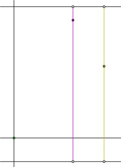
The line segments extending to the right at oblique angles are speed control mechanisms. They control the two points on the colored line segments. Watch closely and you will see that one of them moves back and forth, while the other travels in only one direction. They also move at different speeds. That sounds like a lot of fuss for points that are hidden in the finished sketch. The idea is to simulate random motion. That is not possible, so I settled for unpredictable motion. Their speed is constant, so they do not tend to stay near any particular interval. Therefore we have a uniform distribution. The color of the trace point depends on its position relative to these two points. Move the speed controls to the left to slow things down. Then you will see the pattern better. In this picture, I show only the relationships affecting the color. The red point is the trace point. It is red because it is above both of the points on the colored lines. If it were below both of them, it would be green. If it were between them, it would be blue. This information should make it clear why the trace tends to be red near the top. That is because the higher the trace point goes, the more likely it is to be above both of the color controls.
The trace point is blue if and only if it is between the two control
points. We could compute this one too, but a little bit of reasoning will
save us some work. If the trace point is between the two control points,
then it is not above both of the and it is not below both of them. The
converse of that statement is also true. Therefore the region of success
for blue is simply the complement of the other two regions. It is the two
rectangles not enclosed by either red or green. Its probability is
What if we do not know x? Instead of computing the probabilities for some value of x, let’s find the overall probabilities. If the trace point could be anywhere on its domain, with a uniform distribution, what are the probabilities for the three colors? Without going into great detail on integration, let me show what happens when we make the jump to three dimensions. Lay this same unit square horizontally, and let the height of the square be x. As x goes from 0 to 1, the square fills a unit cube. See the animation below.
The cube can then be broken apart to see its component solids. The red region and the green region are pyramids with square bases. They clearly are congruent. If you examine the symmetry of the problem that started this, you will see why they have to be. The blue region is composed of two tetrahedra.
Back to the Chinese Handcuffs page Last update: April 10, 2026 ... Paul Kunkel whistling@whistleralley.com For email to reach me, the word geometry must appear in the body of the message. |
 What
is the probability? Let the length of the course that is traveled be assigned
an arbitrary value 1. Let x be the distance of the trace point from
the bottom. What is the probability that it is above the control point
on the magenta line? The control point would have to be at a distance less
than x. So a success may be represented by an interval of length
x. The range of possibilities has
What
is the probability? Let the length of the course that is traveled be assigned
an arbitrary value 1. Let x be the distance of the trace point from
the bottom. What is the probability that it is above the control point
on the magenta line? The control point would have to be at a distance less
than x. So a success may be represented by an interval of length
x. The range of possibilities has  Now
compute the probability of the trace point being green. For that to happen,
both of the control points would have to be between x and 1, an
interval of length
Now
compute the probability of the trace point being green. For that to happen,
both of the control points would have to be between x and 1, an
interval of length  Remember,
x is a variable. What we have done here was to compute the probabilities
for any given x in the domain of the trace point. As the trace point
goes up the line, the probability of red goes from 0 to 1 as the red square
grows in size. The probability of green goes from 1 to 0. The probability
of blue is 0 at both ends. Where is its maximum value, and what is that
probability?
Remember,
x is a variable. What we have done here was to compute the probabilities
for any given x in the domain of the trace point. As the trace point
goes up the line, the probability of red goes from 0 to 1 as the red square
grows in size. The probability of green goes from 1 to 0. The probability
of blue is 0 at both ends. Where is its maximum value, and what is that
probability?
 Now you may
or may not know the formula for the volume of a pyramid. The whole point
of this exercise was to see the connection between geometry and probability,
so let’s leave the algebra out of it. In the animated image The two blue
tetrahedra are rotated so that they fit together into a square pyramid
which is congruent to the red and green pyramids. That means that all three
regions have the same volume, and hence, all three colors have the same
overall probability,
Now you may
or may not know the formula for the volume of a pyramid. The whole point
of this exercise was to see the connection between geometry and probability,
so let’s leave the algebra out of it. In the animated image The two blue
tetrahedra are rotated so that they fit together into a square pyramid
which is congruent to the red and green pyramids. That means that all three
regions have the same volume, and hence, all three colors have the same
overall probability,